Article Text

Abstract
Mental health questions can be tackled through machine learning (ML) techniques. Apart from the two ML methods we introduced in our previous paper, we discuss two more advanced ML approaches in this paper: support vector machines and artificial neural networks. To illustrate how these ML methods have been employed in mental health, recent research applications in psychiatry were reported.
- mental health
This is an open access article distributed in accordance with the Creative Commons Attribution Non Commercial (CC BY-NC 4.0) license, which permits others to distribute, remix, adapt, build upon this work non-commercially, and license their derivative works on different terms, provided the original work is properly cited, appropriate credit is given, any changes made indicated, and the use is non-commercial. See: http://creativecommons.org/licenses/by-nc/4.0/.
Statistics from Altmetric.com
Introduction
Machine learning (ML) methods have been increasingly used in mental health and related research. In our last paper, we discussed two ML methods, the logistic regression and the k-means clustering.1 In this report, we focus on two more advanced ML approaches, support vector machines (SVMs) and artificial neural networks (ANNs), along with their applications in psychiatry.
SVM is a supervised learning method to classify labelled outcomes. SVM applies a small number of samples called ‘support vectors’ from each class to build a classifier which separates samples into the different classes.2 SVM is an extension of linear discriminant function, a popular statistical method of supervised learning, as it attempts to accommodate non-linear discriminant functions for more precise classification.3 SVM has been widely used, including in the field of psychiatry. For example, in studies on major depressive disorder (MDD), SVM was employed to identify patients with MDD from healthy controls by using demographic and clinical variables such as age, gender, education level, medication and so on.4 It is also a popular technique in neuroimaging.5 6 We will further discuss SVM in the next section.
ANN is composed of many simple units called ‘artificial neurons’. The main components of ANN are input layers, hidden layers and output layers. Computer scientists have developed ANNs to imitate biological neural networks by building models that mimic the learning process of human brains from training data without any prior knowledge of the data.7 For example, in artificial intelligence, ANNs can be used to learn patterns such as numbers or letters from images (labelled data), then identify these numbers or letters from other images. There is no need to specify the patterns of these numbers or letters a priori or any other characteristics before learning. Thus, ANNs can be used in either supervised learning or unsupervised learning.7 We will focus on its usage in one type of supervised learning—classification—in this paper.
Support vector machine
SVM algorithms are classifiers defined by a particular linear decision boundary called ‘hyperplane’. For simplicity, we assume our data have two classes and are linearly separable, in which case a hyperplane that can perfectly separate the classes exists. In the specific case of two-dimensional feature space, a hyperplane becomes a straight line. Given training data  , where
n
is the sample size,
d
is the number of predictors, and
, where
n
is the sample size,
d
is the number of predictors, and  denotes the
d
-dimensional Euclidean space, the goal of SVM is to find a hyperplane that can split the data points into the two classes. Note that the hyperplane can be written as
denotes the
d
-dimensional Euclidean space, the goal of SVM is to find a hyperplane that can split the data points into the two classes. Note that the hyperplane can be written as  and
and  , so we want to find
w
and
b
such that
, so we want to find
w
and
b
such that  for all
i
. By scaling
w
and
b
, it is equivalent to finding
w
and
b
such that
for all
i
. By scaling
w
and
b
, it is equivalent to finding
w
and
b
such that  for all
i
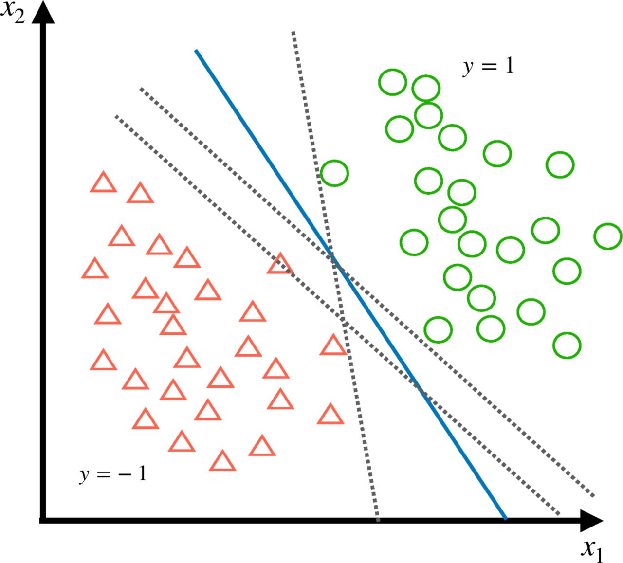
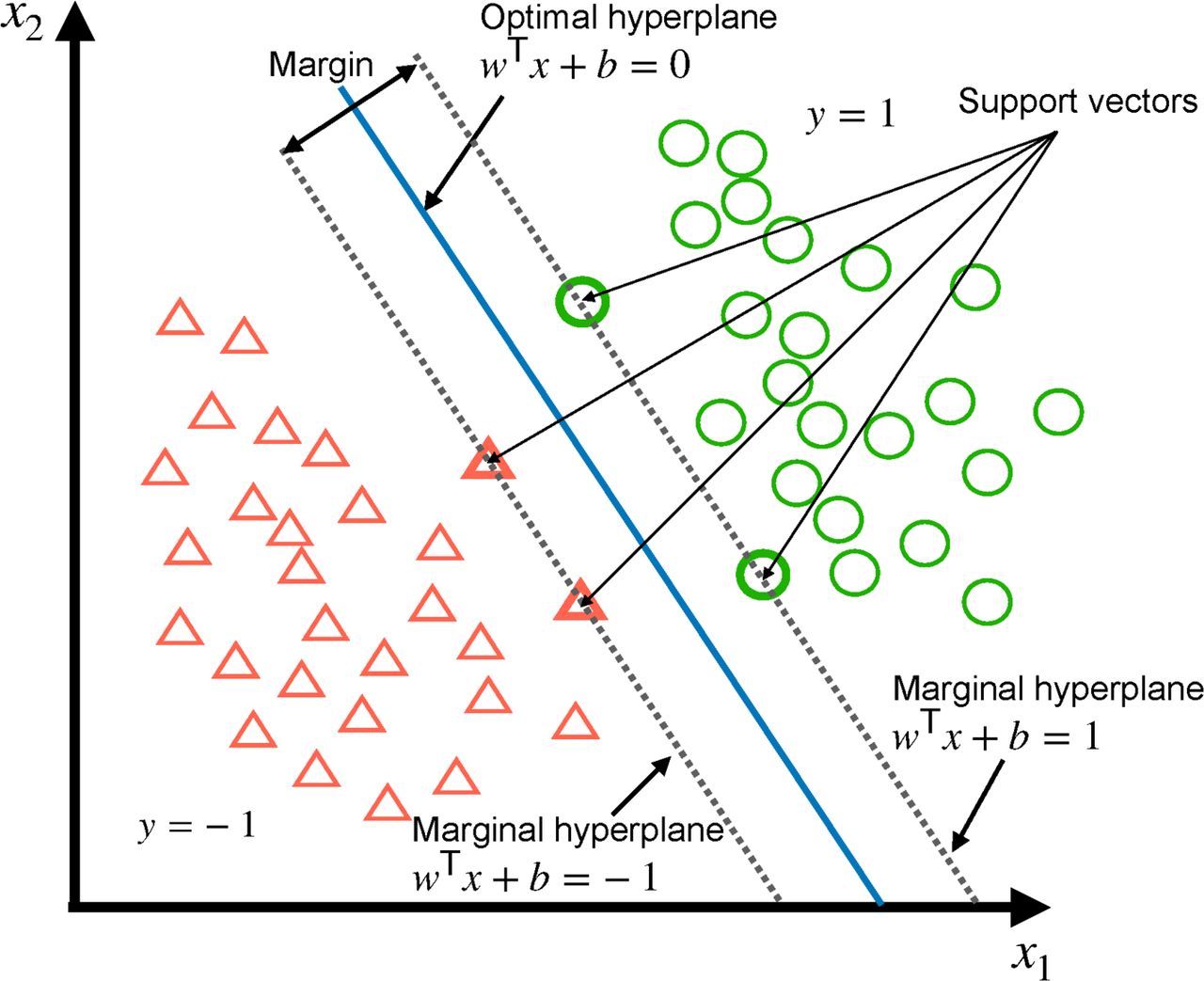
. There are infinitely many hyperplanes that can achieve our goal if the data are linearly separable (figure 1). To increase the possibility that the hyperplane is a ‘good’ classifier not only for the training data, we desire to have a hyperplane that can be as far as possible from the both classes, which means the best hyperplane is the one that lies ‘in the middle’ of the two classes (figure 2). In order to find such hyperplane, the problem becomes to maximise the distance from the hyperplane to the nearest data points in each class. It turns out that these nearest data points, or support vectors, can be found to completely determine such an optimal hyperplane.8
for all
i
. There are infinitely many hyperplanes that can achieve our goal if the data are linearly separable (figure 1). To increase the possibility that the hyperplane is a ‘good’ classifier not only for the training data, we desire to have a hyperplane that can be as far as possible from the both classes, which means the best hyperplane is the one that lies ‘in the middle’ of the two classes (figure 2). In order to find such hyperplane, the problem becomes to maximise the distance from the hyperplane to the nearest data points in each class. It turns out that these nearest data points, or support vectors, can be found to completely determine such an optimal hyperplane.8

There are many hyperplanes that can split the data into two classes if the data are linearly separable.

The linearly separable case where the optimal hyperplane separates the data into two-dimensional feature space.
In practice, data are often not linearly separable. In this case, we can allow some points to lie on the wrong side of their ‘marginal hyperplane’—a hyperplane that is parallel to the optimal hyperplane and passed through support vectors. The region bounded by the two marginal hyperplanes is called the ‘margin’. We define the ‘slack variable’ of a data point as the distance of such point to its marginal hyperplane if the point lies on the wrong side of its marginal hyperplane, and zero if it lies on the correct side of its marginal hyperplane (figure 3). This approach may not work for classes that are truly non-linear. For example, if one class is inside and the other is outside a circle, this ad-hoc approach will not work. A qualitative improvement by SVM over the classic linear discriminant method is the ‘kernel trick’.8 In this case, we apply kernels, or mathematical transformations, to transform data points observed in the study into data points in a higher dimensional Euclidean space and consider separation of classes by determining a hyperplane in such high dimensional space. There is no guarantee that there exists a kernel function to achieve perfect separation in every application. Even if such a kernel exists, finding it is no means straightforward. Nonetheless, SVM in theory offers new opportunities and more choices for better classifiers than its classic counterparts such as the linear discriminant function.

The non-linearly separable case where the optimal hyperplane separates the data into two-dimensional feature space. Note that  are positive slack variables of the data.
In a recent study, Mikolas et al . 6 applied linear SVM to brain fractional anisotropy (FA) data consisting of 77 first episode of schizophrenia-spectrum disorder (FES) and 77 healthy controls (HC). They were interested in whether SVM would identify the FES from the HC based on the preprocessed skeletonised FA images. If we allow some data points to be misclassified by SVM (slack) and assume the label of FES is 1 and the control is −1, then the optimisation problem can be formulated as follows:

Subject to  and
and  for all
i
, where
for all
i
, where  is a vector of voxels of the
i
th image,
is a vector of voxels of the
i
th image,  is a vector of the slack variable for each point, and
C
is a parameter that controls the trade-off between the margin size and the total error
is a vector of the slack variable for each point, and
C
is a parameter that controls the trade-off between the margin size and the total error  . Note that, by definition, slack variables are always non-negative. If data are linearly separable, then
  , and the problem is the same as the linear separable case described above. For the parameter
C
, a larger
C
means a larger weight of slack, or a smaller margin, resulting in less misclassified points. A smaller
C
provides a larger margin and allows more points to be misclassed. To determine what
C
to use, one can use a grid search method and cross-validation to choose a
C
that has the smallest cross-validation error.9 After estimating
w
and
b
, we determine a hyperplane for classification. Given
, and the problem is the same as the linear separable case described above. For the parameter
C
, a larger
C
means a larger weight of slack, or a smaller margin, resulting in less misclassified points. A smaller
C
provides a larger margin and allows more points to be misclassed. To determine what
C
to use, one can use a grid search method and cross-validation to choose a
C
that has the smallest cross-validation error.9 After estimating
w
and
b
, we determine a hyperplane for classification. Given  as a new image data point, if
  is positive, we classify the new image as FES, otherwise we classify it as control.
Artificial neural network
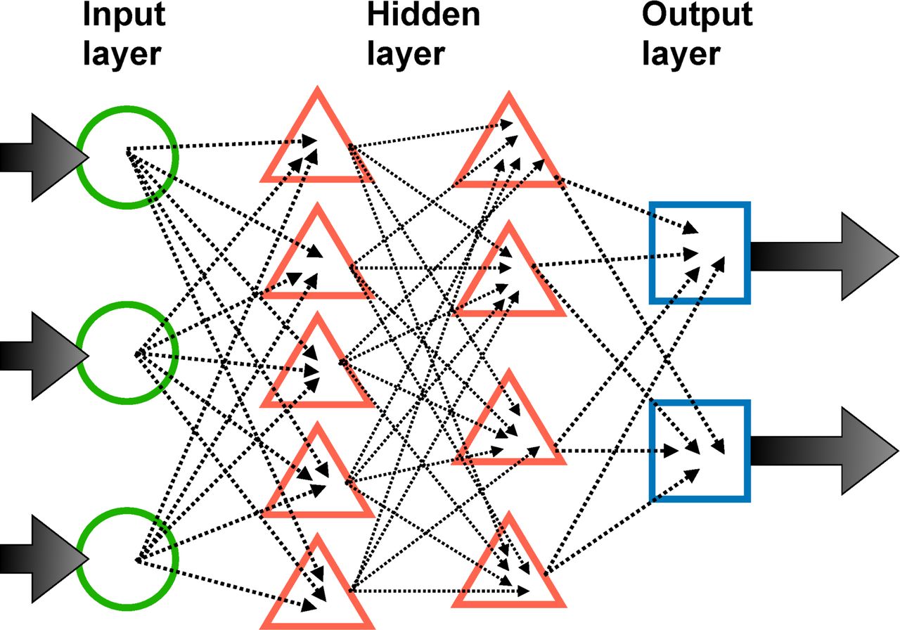
Like a human brain, ANN comprised artificial neurons. Artificial neurons receive inputs, process the information (compute a weighted sum of the inputs and maps it into a non-linear function called activation function) and produce an output.7 From the viewpoint of biology, the inputs correspond to the signal received by the dendrites, the processing of inputs corresponds to the soma, and the outputs correspond to the signal transmitted from the axon. The outputs will be the inputs of the next artificial neurons, thus forming a network. Activation functions can be viewed as rules of transmitting the signal. In the soma, when the electrical potential reaches a certain threshold, a signal pulse will be transmitted by the axon. Common activation functions include step function, sigmoid (logistic) function and rectified linear unit.10 When describing an ANN model, each artificial neuron can be considered as a node. If the output of an artificial neuron is the input of another artificial neuron, we can connect these two nodes by an arrow. The connections can be assigned different weights to represent different importance. There is no restriction on the number of connections. One node can have multiple inputs from other nodes and multiple outputs transmitted to others. The collection of artificial neurons that receive inputs from training data is called the input layer, which is the first layer of the ANN model. Similarly, the collection of neurons that produce final outputs is called the output layer, which is the final layer of the ANN model. The other neurons that do not belong to the above two layers are in hidden layers. The number of hidden layers depends on the problem we are trying to solve, therefore the structure of connections varies from case to case. The first and the simplest type of ANN is a feedforward neural network (FNN) in which neurons in each layer feed their outputs forward to the next layer until the final outputs.11 12 FNN only has one direction of information transmission without any feedback such as cycles or loops (figure 4).

An example of a feedforward neural network.
A common class of FNN is the multilayer perceptron (MLP). The perceptron is defined as a function
f
called Heaviside step function that maps input  to a binary output

where  is a vector of weights and
  is the bias.13 MLP is composed of many perceptions, but the function defined in the perceptron can be placed by other activation functions such as sigmoid, Gaussian and so on.14 Different activation functions allow MLP to perform either classification or regression. In psychiatry, MLP can be applied to brain imaging data. Wang et al.15 used MLP to identify Alzheimer’s disease from brain MRIs. MLP is typically trained by backpropagation (BP) algorithm. The goal of BP is to find
w
and
b
that minimise the loss function (eg, squared loss) by gradient methods such as gradient descent. BP computes the gradient of the loss function with respect to
w
and
b
by the chain rule, and updates them in each of the iteration until the error between the network output and the actual output is smaller than a preassigned threshold.16
is the bias.13 MLP is composed of many perceptions, but the function defined in the perceptron can be placed by other activation functions such as sigmoid, Gaussian and so on.14 Different activation functions allow MLP to perform either classification or regression. In psychiatry, MLP can be applied to brain imaging data. Wang et al.15 used MLP to identify Alzheimer’s disease from brain MRIs. MLP is typically trained by backpropagation (BP) algorithm. The goal of BP is to find
w
and
b
that minimise the loss function (eg, squared loss) by gradient methods such as gradient descent. BP computes the gradient of the loss function with respect to
w
and
b
by the chain rule, and updates them in each of the iteration until the error between the network output and the actual output is smaller than a preassigned threshold.16
Discussion and conclusion
In this paper, we introduced two advanced ML approaches and their applications in mental health and related fields. Compared with logistic regression and k-means clustering, the final models of SVM and ANN are usually more difficult to understand and interpret, which is especially true for ANN, as it does not directly correspond to any statistical methods. However, these two methods work well with unstructured data such as images and texts, for which statistical methods are seldom used. As imaging analysis and text mining all have applications in mental health and related research, we believe that an understanding of the components and capabilities of these and other advanced ML methods will help to develop an appreciation of their existing and potential applications and apply them to improve our understanding and treatment of mental disorders.
References
Tsung-Chin Wu is a second year master’s student studying statistics at University of California, San Diego (UCSD). He works at the Sam and Rose Stein Institute for Research on Aging in UCSD as a Graduate Student Researcher. He obtained both a Bachelor of Science degree in Mathematics and a Bachelor of Science degree in Horticulture and Landscape Architecture at National Taiwan University. Tsung-Chin has a strong interest in modern statistical applications for mental health data, and has applied many statistical methods for longitudinal data analysis, causal inference, and machine learning.

Footnotes
Contributors T-CW and ZZ conceived of the presented idea. T-CW wrote the manuscript with support from ZZ, HW, BW and TL. CF and XMT helped supervise the project.
Funding The authors have not declared a specific grant for this research from any funding agency in the public, commercial or not-for-profit sectors.
Competing interests None declared.
Patient consent for publication Not required.
Provenance and peer review Commissioned; internally peer reviewed.