Post-hoc power analysis for comparing two population means

Within the power analysis paradigm, the reason why post-hoc power analysis is conceptually flawed is the misinterpretation of parameters for power analysis in prospective studies. In fact, standard power analysis is ill-posed for assessing the reliability of significant statistical findings from data of a completed study. We discuss one more appropriate formulation that extends the current power analysis paradigm to address the fundamental flaw in the existing approach.

For convenience, consider two independent samples and let Y _ik denote a continuous outcome of interest from subject i and group . For simplicity and without loss of generality, we assume that for both groups Y _ik follows a normal distribution population mean and common population variance , denoted . The most popular hypothesis for comparing two groups is whether the population means are the same between the two groups, that is:

(1)

where δ is a known constant and H ₀ (H _a) is known as the null (alternative) hypothesis. The hypothesis in Equation 1 is known as a two-sided hypothesis as no direction of effect is specified in the alternative hypothesis H _a. If a directional effect is also indicated, such as in Equation 2, the hypothesis is called a one-sided hypothesis.

(2)

In addition to stating that the two population means are different, it also indicates that the population mean for group 1 is larger (or smaller) than that for group 2 under the alternative. Since two-sided hypotheses are much more popular in practice, we focus on the two-sided hypothesis throughout the rest of the discussion unless stated otherwise. However, all results and conclusions derived apply to the one-sided hypothesis.

Note that when testing the hypothesis in Equation 1 as in data analysis, δ is an unknown constant and p values are calculated based on the null H ₀ without any knowledge about δ in the alternative H _a. For power analysis, however, this mean difference must be specified, which actually is the most important parameter for power analysis.

In practice, the normalised difference, or Cohen’s , is often used since it is invariant under linear transformation.6 This invariance property plays a significant role in statistical analysis. For example, consider comparing gas mileage between two types of vehicles, such as sport utility vehicles (SUVs) and sedans. If this study is conducted in the USA, miles per gallon of gas will be used to assess gas mileage for each vehicle. If the study is conducted in Canada, kilometres per gallon of gas will be used to record gas mileage for each car. Although the means for the two classes of vehicles are different, the effect size is the same regardless of whether kilometres or miles are used to measure distance travelled per gallon of gas. With the unitless effect size, the hypothesis in Equation 1 can be expressed as:

(3)

We will use effect size d and the hypothesis in Equation 3 in what follows unless stated otherwise.

Note that all popular statistical models such as t-tests and linear regression have the invariance property under linear transformation so that the same level of statistical significance is reached regardless of measurement units used. For example, in the above gas mileage example, if we model the outcome of miles travelled per gallon of gas as a function of manufacturers in addition to differences between SUVs and sedans using linear regression, we will get different estimates of regression parameters (coefficients) and standard errors, but same test statistics (F and t statistics) and p values.

In clinical research, the magnitude of d is used to indicate meaningful treatment difference or exposure effects. This is because statistical significance is a function of sample size and any small treatment difference can become statistically significant with a sufficiently large sample size. Thus, statistical significance cannot be used to define the magnitude of treatment or exposure effects. Defined only by the population parameters, effect size is a meaningful measure of the magnitude of treatment or exposure effects. Equation 3 indicates that both the null and alternative hypotheses only involve population parameters. This characterisation of the statistical hypothesis is critically important since this fundamental assumption is violated when performing post-hoc power analysis.

For power analysis, we want to determine the probability to reject the null H ₀ in favour of the alternative H_a under H_a for the hypothesis in Equation 3. To compute power, we need to specify the H ₀, H_a , type I error α, and sample size n ₁ and n ₂, with n _k denoting the sample size for group k (k=1,2). Given these parameters, power is the probability of rejecting the null H ₀ when the alternative H_a is true:

(4)

where Pr(A|B) denotes the conditional probability of the occurrence of event A given event B, Z denotes a random variable following the standard normal distribution N(0,1), Z _α/2 denotes the upper α/2 quantile of N(0,1), and denotes the cumulative distribution function of the standard normal distribution N(0,1). If we condition on the null H ₀ instead of H _a in Equation 4, we obtain a type I error, as in Equation 5:

(5)

which is the probability of rejecting the null H ₀ when the null is true. For power analysis, we generally set type I errors at α=0.05, so that Z _α/2 =Z _0.025=1.96.

In practice, we often set power at some prespecified levels and then perform power analysis to determine the minimum sample size to detect a prespecified effect size Δ with the desired level of power. For example, if we want to determine sample size n per group to achieve, say, 0.8 power with equal sample between two groups, we can obtain such minimum n by solving for n in the following equation7:

(6)

When applying Equation 3 for a post-hoc power analysis in a study, we substitute the observed effect size in place of the true effect size Δ. This observed is calculated based on the observed study data with sample size n ₁ and n ₂:

where is the sample mean of group k and s _n is the pooled sample standard deviation (SD):

Unlike Δ, the observed effect size is computed based on a particular sample in the study and thus subject to sampling variability. Unless for an extremely large sample size, may deviate substantially from Δ. Thus, power is calculated based on :

(7)

Equation 7 only indicates the probability to detect the sample effect size , which can be quite different from power estimates computed based on the true population effect size Δ. Except for large sample sizes n, power estimates based on can be highly variable, rendering them uninformative about the true effect size Δ.

On the other hand, post-hoc power analysis based on Equation 7 also presents a conceptual challenge. Under the current power analysis paradigm, power is the probability to detect a population-level effect size Δ. This effect size is specified with complete certainty. For example, if we set Δ=0.5, it means that we know that the difference between two population means of interest is 0.5. For post-hoc power analysis, we compute power using as if this was the difference between the two population means. Due to sampling variability, varies around Δ and the two can be substantially different. Indeed, as illustrated in Zhang et al,1 post-hoc power based on Equation 7 can be misleading when used to indicate power for Δ based on Equation 4.

Thus, for post-hoc power analysis to be conceptually consistent with power analysis for prospective studies and informative about the population effect size Δ, we must account for the sampling variability in . Although , is generally informative about Δ, with diminishing uncertainty as sample size increases, a phenomenon known as the central limit theorem (CLT) in the theory of statistics.8 By quantifying the variability in and incorporating such variability in specifying the alternative hypothesis, we can develop new post-hoc power analysis to inform our ability to detect Δ.

By the CLT, the variability of is described by a normal distribution . Thus, in the absence of knowledge about Δ, values closer to are better candidates for Δ, while values more distant from are less likely to be good candidates for Δ. By giving more weights to values closer to and less weights to values more distant from , the normal distribution centred at , , quantifies our uncertainty about Δ. Thus, for post-hoc power analysis, we replace the alternative hypothesis in Equation 3 involving a known population effect size Δ with a set of candidate values for Δ with their candidacy described by the distribution :

(8)

The hypothesis in Equation 8 is fundamentally different from the hypothesis in Equation 3 for regular power analysis for prospective studies. Unlike Equation 3, there are more than one candidate value for Δ and post-hoc power analysis must consider all such candidate ds with their relative informativeness for Δ described by the distribution . Thus, a sensible way to achieve this is to average power estimates over all such candidates according to their relative informativeness for Δ described by the distribution . However, since there are infinitely many such Δs, we need to use integrals in calculus to perform this averaging.

Let denote the density function of the normal distribution . Then by averaging the power function in Equation 7 over all plausible values of Δ weighted by the distribution , we obtain power for the hypothesis in Equation 8:

(9)

where denotes the value of the integral of the function over the interval .

In the new formulation of hypothesis in Equation 8, we essentially treat true effect size d as a random variable, rather than a (known) constant as under the current power analysis paradigm. This perspective by viewing unknown population parameters as random variables is not new and in fact a well-established statistical paradigm known as Bayesian inference. Under this alternative paradigm, the choice about an unknown population parameter such as d within the current context does not have to be an unknown constant, but can vary over a range of possibilities following a distribution that reflects our knowledge about the true d. For example, in the hypothesis in Equation 8, our knowledge about d is informed by an observed , with its variability described by the normal distribution . In contrast, the traditional hypothesis for post-hoc power analysis in Equation 7 treats as the absolute truth, which completely violates the fundamental assumption of the power analysis paradigm.

The new formulation also allows one to build up knowledge about d. For example, if we use a distribution to describe our knowledge about d prior to an observed based on the study data, we can then integrate our a priori knowledge with to obtain a distribution to describe our improved knowledge about d and use it in Equation 8. This improved knowledge about d obtained by combining our initial knowledge with observed from a real study is known as a posterior distribution. The distribution that describes our initial knowledge is called a prior distribution. By using a posterior distribution as a new prior with data from an additional study, we can derive a new posterior distribution. We can keep updating our knowledge by repeating this process.

For example, within the current study context, we may start without any knowledge about d, in which case we can use a non-informative prior distribution, or a constant. After obtaining from a real study with sample size n=n ₁+n ₂, our posterior is . If there is a new from an additional study about d with sample size m=m ₁+m ₂, we then obtain a new posterior distribution that integrates information from both observed and , which is still a normal but with a different mean and variance , where and are given by:

(10)

By setting m ₁=m ₂=0, the above normal reduces to . To see this, first set m ₁=m ₂=m, then simplify and in Equation 10 to:

(11)

Setting m=0, the and in Equation 11 reduce to and . Thus, we may view a non-informative prior as an observed from a study with zero sample size.

Illustrations

In this section, we use Monte Carlo simulation to compare the three types of power analysis, that is, the regular power analysis for a prospective study in Equation 4 and the two post-hoc power analyses with one based on observed effect size in Equation 7 and the other on the new paradigm in Equation 8. In all cases, we set a two-sided alpha at α=0.05 and Monte Carlo sample size at 1000.

We again assume a normal distribution , with denoting the (population) mean of group k and σ ² the common (population) variance. We set the population parameters as follows:

(12)

Since σ ²=1, the difference between the means, Δ, is Cohen’s d, which is interpreted as Δ=0.2, Δ=0.5 and Δ=0.8 for small, medium and large effect size, respectively.6 For convenience, we assume a common sample size for both groups, that is, n ₁=n ₂=n. We set Δ and n to different values so we can see how power estimates from the three different approaches change as a function of the two parameters.

Given all these parameters, we can readily evaluate the prospective power function in Equation 6. For post-hoc power analysis, power is not a constant and varies according to observed effect size . We use Monte Carlo simulation to capture such variability. Given the parameters in Equation 12 and sample size n, we simulate sample, , from , compute the sample effect size and evaluate the post-hoc power functions in Equation 7 and Equation 9. Thus, unlike prospective power, both post-hoc power functions depend on the observed effect size . The difference is that Equation 7 treats as the true effect size, while Equation 9 acknowledges sampling variability in and uses its sampling distribution to inform the underlying effect size Δ.

The variance of is , which will be close to 0 and will be close to Δ for a very large sample size n. In this case, both post-hoc power will be close to the prospective power. For small and moderate sample sizes, all three power values will differ from each other. Given Δ, the prospective power only has one value for each sample size, while the two post-hoc power approaches will have different values for different observed . For small and moderate sample sizes, post-hoc power values will have large variabilities and may not be informative about the power based on the true Δ.

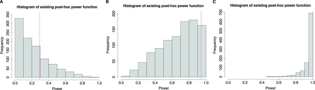
Shown in figure 1 are the histograms of power from the existing post-hoc power approach based on 1000 Monte Carlo sample sizes for effect size Δ=0.2 (figure 1A), Δ=0.5 (figure 1B) and Δ=0.8 (figure 1C), along with power from the prospective power function (vertical line) for sample size n=50. As expected, power increased in both cases as the true effect size Δ became larger; the sample mean for the post-hoc power was 0.167, 0.443 and 0.761, respectively. For all three effect sizes, there was a large amount of variability in the post-hoc power, covering the entire range of power function between 0 and 1.

• Download figure
• Open in new tab
• Download powerpoint

Figure 1

Histogram of power from existing post-hoc power function, along with power from the prospective power function for sample size n=50, based on 1000 Monte Carlo runs for effect size (A) Δ=0.2, (B) Δ=0.5 and (C) Δ=0.8.

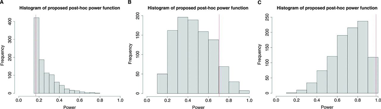
Shown in figure 2 are the histograms of power from the proposed post-hoc power approach based on 1000 Monte Carlo sample sizes with the mean difference Δ=0.2 (figure 2A), Δ=0.5 (figure 2B) and Δ=0.8 (figure 2C), along with power from the prospective power function (the vertical line) for sample size n=50. As in figure 1, the mean power increased from 0.259 to 0.463 to 0.711 when Δ changed from 0.2 to 0.5 to 0.8. Unlike in figure 1, power was larger than 0.1 in all three cases. Moreover, the sample SDs for the three effect sizes were 0.111, 0.177 and 0.162 for the proposed, compared with 0.151, 0.239 and 0.194 for the traditional power method. The smaller variability of the proposed post-hoc power was the result of being less sensitive to variability in , compared with the existing post-hoc power.

• Download figure
• Open in new tab
• Download powerpoint

Figure 2

Histogram of power from a proposed post-hoc power function, along with power from the prospective power function for sample size n=50, based on 1000 Monte Carlo runs for effect size (A) Δ=0.2, (B) Δ=0.5 and (C) Δ=0.8.

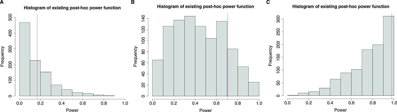
Shown in figure 3 are the histograms of power from the existing post-hoc power approach based on 1000 Monte Carlo sample sizes for effect size Δ=0.2 (figure 3A), Δ=0.5 (figure 3B) and Δ=0.8 (figure 3C), along with power from the prospective power function (the vertical line) for sample size n=100. As in figure 1, as Δ changed from 0.2 to 0.5 to 0.8, the mean power increased from 0.226 to 0.670 to 0.951. Again, post-hoc power was quite variable, covering the entire range in all cases, except for Δ=0.8, where the minimum was 0.48. With Δ=0.8 and n=100, the smaller sampling variability along with the large effect size led to power values close to 1, greatly reducing the variability of post-hoc power, as compared with n=50.

• Download figure
• Open in new tab
• Download powerpoint

Figure 3

Histogram of power from existing post-hoc power function, along with power from the prospective power function for sample size n=100, based on 1000 Monte Carlo runs for effect size (A) Δ=0.2, (B) Δ=0.5 and (C) Δ=0.8.

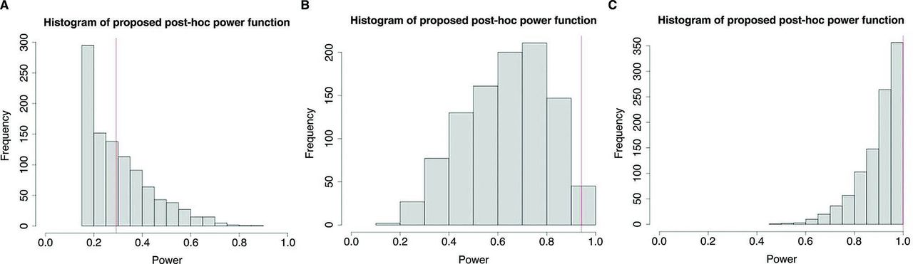
Shown in figure 4 are the histograms of power from the proposed post-hoc power approach based on 1000 Monte Carlo sample sizes with the mean difference Δ=0.2 (figure 4A), Δ=0.5 (figure 4B) and Δ=0.8 (figure 4C), along with power from the prospective power function (the vertical line) for n=100. As in figure 3, the mean power grew from 0.303 to 0.636 to 0.901 as Δ increased from 0.2 to 0.5 to 0.8. The sample SDs for Δ=0.2, Δ=0.5 and Δ=0.8 were 0.135, 0.174 and 0.086, compared with 0.184, 0.221 and 0.071 for the existing power in figure 3. Except for Δ=0.8, the proposed post-hoc power was less variable than its existing counterpart. For Δ=0.8, the trend was reversed and post-hoc power was more variable for the proposed than the traditional approach. This is made clear by comparing the two histograms in figure 3C and figure 4C. For Δ=0.8, there was much less variability in power from the traditional than the proposed approach; about 70% of power values were between 0.95 and 1 for the traditional approach, compared with about 30% for the proposed approach. Thus, this smaller variability of power from the traditional approach again reflects its higher sensitivity to the observed than the proposed alternative.

• Download figure
• Open in new tab
• Download powerpoint

Figure 4

Histogram of power from proposed post-hoc power function, along with power from the prospective power function for sample size n=100, based on 1000 Monte Carlo runs for effect size (A) Δ=0.2, (B) Δ=0.5 and (C) Δ=0.8.