Power analysis for comparing two population Means

We have considered to use two independent samples and let Y _ik denote a continuous outcome of interest from subject i and group k (1≤i≤n _k, k=1,2). For simplicity and without loss of generality, we assume that for both groups, Y _ik follows a normal distribution of population mean μ _k and common population variance σ ², denoted as

The most common hypothesis in this setting is whether the population means are equal to each other. In statistical lingo, we state the hypothesis as follows:

(1)

where δ is a known (unknown) constant for power (data) analysis, and H ₀ and H _a are known as the null and alternative hypotheses, respectively. The above is known as a two-sided hypothesis, as no direction of effect is specified in the alternative hypothesis . If the directional effect is also indicated, the alternative becomes a one-sided hypothesis. For example, if the alternative is specified as: , it is one sided and μ ₁ is hypothesised to be larger than μ ₂ under H _a. As two-sided alternatives are the most popular in clinical research, we only consider two-sided alternatives in this paper unless stated otherwise. Note also that when testing the hypothesis in equation (1) with data as in data analysis, δ is an unknown constant and p values are calculated based on the null H ₀ without any knowledge about δ in the alternative H _a. For power analysis, the difference δ must be specified, since power depends on this parameter. In practice, the normalised difference, , is often used, as it is more succinct and generally has a more meaningful interpretation. This normalised difference is known as Cohen’s d.1

The hypothesis in equation (1) is generally tested using the two sample t-test. Let denote the sample mean of the kth group (k=1,2). The difference between the two sample means should be close to 0 if H ₀ is true. Again, because and are random, it is still possible for to be very different from 0, although such probabilities are small, especially for large sample size n, a statistical result known as the law of large numbers.7 To address this sampling variability in causing wrong conclusions about the hypothesis, type I error, typically denoted by α, is used to indicate the extent to which the difference, , departs from 0. This error rate is typically set at α=0.05 for most studies. For very large sample sizes, α is generally set at a more stringent level, α=0.01. Given α, power is the probability that H ₀ is rejected when H _a in fact is true.

If is true, the probability of rejecting H ₀, therefore committing type I error a, is the probability:

(2)

where z _{α /2} is the upper α/2 quantile of the standard normal distribution, P(A) denotes the probability of the occurrence of an event A and s is the pooled SD:

The probability in equation (2) is readily evaluated using the t distribution.

Note that like the effect size, the difference between the sample means in equation (2) has also been normalised (by the pooled SE) so that the type I error a does not depend on other artefacts such as different scales that may be used for the outcomes. Note also that we assume a common SD (or variance) between the groups for the t-statistic in equation (2). If this is not the case, we can use the version of the two sample t-test for unequal variances, called the Welch’s t-test. For simplicity and without loss of generality, we focus on the equal variance version in equation (2) in what follows. The same conclusions also apply to the Welch’s t-test.

For power analysis, we want to determine the probability to reject the null H ₀ in favour of the alternative H _a. Given the type I error α, sample size n ₁ and n ₂, and H ₀ and H _a, we can calculate power for reject the null H ₀:

(3)

Although similar in apperance, equation (3) is actually quite different from equation (2). equation (2) is generally used to compute p values, in which case and s are all readily computed from the sample means and sample SD from the observed outcomes. As none of these quantities is available when performing power analysis for prospective studies, the power function in equation (3) is evaluated based on sample sizes, n ₁ and n ₂, the population mean difference δ and SD σ. Thus, unlike data analysis, all these parameters must be explicitly specified in order to compute power. Although results from similar studies may be used to help suggest and specify δ and σ, they are both conceptually and analytically different from their sample counterparts. Conceptually, δ and σare determined by the entire study population, while δ and s are specific to a random sample from the study population. Analytically, δ and σ are population-level constants, whereas δ and s are random quantities and vary from sample to sample. The population parameters can be quite different from their sample counterparts.

In practice, we often set power at some prespecified levels and then perform power analysis to determine the minimum sample size to achieve the desired levels of power. We can use the power function equation (3) for this purpose as well. For example, if we want to determine sample sizes n ₁ and n ₂ to achieve, say, 0.8 power, we can solve for n ₁ and n ₂ in the following equation:8

(4)

Note also that power functions can also be evaluated by replacing the mean difference δ and SD σ with the composite effect size d. Unlike δ, d is unit free and well interpreted, with d=0.2, 0.5 and 0.8 representing small, medium and large effect size.1

Post hoc power analysis for comparing two population means

In the preceding section, we discussed power analysis for comparing two population means for prospective studies. To evaluate power, we must specify the mean difference between the two population means, regardless of whether we want to estimate power for the given sample size or vice versa. Such a difference is study specific, which, although may be suggested by similar studies, should not be exclusively determined by one single study. This is because unlike the difference between population means δ, difference calculated based on a particular study sample δ is random and can be quite different from δ. As a result, power or sample size determined from sample-based mean difference δ can be quite different from the true power for prospective studies.

The difference between the population and sample-based parameters underscores the problem with post hoc power analysis. Not only is power analysis performed based on the sample-based mean difference, power estimates are also applied back to the same data to indicate power. Post hoc power analysis identifies population-level parameters with sample-specific statistics and makes no conceptual sense. Analytically, such analysis can yield quite different power estimates that are difficult and can be misleading.

To see this, consider again the problem to test the hypothesis in equation (1). Following the discussion in the preceding section, we can use equation (3) to computer power or use equation (4) to determine sample size for a desired level of power. When calculating power or sample size for post hoc analyses for a study with the outcomes already observed, the mean difference δ and SD σ will be set to their sample-based counterparts. Let and denote the sample means, and s denote the pooled sample SD from the study sample. By replacing δ with and σ with s in equation (3), we obtain the power function for post hoc power analysis.

To help see the difference, we express the two power function side-by-side as follows:

(5)

The prospective power function is determined by the population mean difference δ and SD σ, but the post hoc power function depends on the sample mean difference δ and sample SD s. For large sample sizes, both δ and s will be close to their respective population counterparts, which is guaranteed by the law of large numbers. However, for relatively small sample sizes, δ, s or both can become quite different from their respective population parameters, in which case the two power functions in equation (5) can yield very different values. Next, we use simulation studies to compare performance of the two power functions.

Illustrations

In this section, we use Monte Carlo simulation to compare the prospective and post hoc power functions. In all cases, we set a two-sided alpha at α=0.05 and Monte Carlo sample size at 1000.

We again assume a normal distribution for the outcomes Y _ik, with μ _k denoting the (population) mean of group k and σ ² the common (population) variance. We set the population-level parameters as follows:

For convenience, we assume a common sample size for both groups, that is, n ₁=n ₂=n. We set δ and n to different values so we can see how the two power functions change for different effect size and sample size.

Given all these parameters, we can readily evaluate the prospective power function in equation (5). For post hoc power analysis, we simulate a sample from the normal distributions, compute the sample mean difference δ and sample SD s based on the simulated outcomes and evaluate the post hoc power function in equation (5). Unlike its prospective counterpart, this power function depends on the particular sample simulated. If δ and s are close to δ and σ, the two power functions will be close to each other. As indicated earlier, this will be the case for large sample sizes thanks to the law of large numbers. For relatively small samples, δ, s or both can be quite different from their population counterparts, in which case using the post hoc power function to informative power can be misleading.

With Monte Carlo simulation, we can readily examine the difference between the two power functions. By repeatedly simulating samples from the population distributions, we can look at the variability of the post hoc power function and see how it performs with respect to predicting true power.

Shown in figure 1 are the histograms of the post hoc power function based on 1000 Monte Carlo sample sizes with the mean difference δ=0.5 (figure 1A), δ=1 (figure 1B) and δ=2 (figure 1C) and n=50, along with the power from the prospective power function (the vertical line segment). As expected, the true power increases as the mean difference δ becomes large. For δ=2, true power is close to 1 and there is not much variability in the post hoc power function. For the other two values of δ, there is quite a large amount of variability in the post hoc power, covering the entire power function range between 0 and 1. The direction of skewness of the histogram changes from right skewed for δ=0.5 to left skewed for δ=1 to more left skewed at δ=2. Unless the true power is at its upper bound 1, post hoc power is too variable to be informative for the true. For δ=2, although there is not much variability, post hoc power is not really informative for any piratical purposes either, since the true power is close to 1.

• Download figure
• Open in new tab
• Download powerpoint

Figure 1

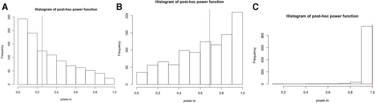
Histograms of post hoc power, along with true power, based on 1000 Monte Carlo sample sizes with the mean difference: (A) δ=0.5; (B) δ=1 and (C) δ=2 and a sample size n=50.

Shown in figure 2 are three histograms of the post hoc power function based on the same parameters, but with a large sample size n=100. Both the prospective and post hoc power functions show the same patterns as observed in figure 1, as δ increases. Even with the true power close to 1 in the case of δ=1, there is still variability in the post hoc function as shown in figure 2B.

• Download figure
• Open in new tab
• Download powerpoint

Figure 2

Histograms of post hoc power, along with true power, based on 1000 Monte Carlo sample sizes with the mean difference: (A) δ=0.5, (B) δ=1 and (C) δ=2 and a sample size n=100.