Article Text

Abstract
Sample size justification is a very crucial part in the design of clinical trials. In this paper, the authors derive a new formula to calculate the sample size for a binary outcome given one of the three popular indices of risk difference. The sample size based on the absolute difference is the fundamental one, which can be easily used to derive sample size given the risk ratio or OR.
- odds ratio
- relative risk
- risk difference
This is an Open Access article distributed in accordance with the Creative Commons Attribution Non Commercial (CC BY-NC 4.0) license, which permits others to distribute, remix, adapt, build upon this work non-commercially, and license their derivative works on different terms, provided the original work is properly cited and the use is non-commercial. See: http://creativecommons.org/licenses/by-nc/4.0
Statistics from Altmetric.com
Introduction
Sample size calculation is an essential part in the design of clinical trials. In many cases, a primary outcome of interest is compared between two groups (namely control and treatments groups) in a trial. Usually, the sample size calculation is related to the test statistic used in such comparisons. However, as discussed in section 2, more assumptions are needed to uniquely determine the sample size.
Suppose we want to design a clinical trial to determine if the treatment effect of a new drug is better than that of the current one. The most popular design is to assign patients randomly to the treatment group (the new drug) and the control group (current drug). If the outcome is a success or a failure, it is a binary variable. Generally, for binary outcomes, there are three popular measures of treatment difference: risk difference, relative risk and OR.1 See Feng and colleagues2 for relationships among these three measures of effect size.
Formulas for sample size estimation for the binary outcome has been well developed and incorporated in many statistical software packages. See, for example, the formula of Chow and colleagues3 (4.2.2). In this paper, the authors derive another formula using more information in the hypotheses. Once the sample size formula based on risk difference is obtained, the sample size formulas for the other two indices can be acquired easily.
In this paper, the authors consider the sample size calculation in the parallel design. This paper is organised as follows. In section 2, the authors derive a new formula based on the null hypothesis of the success rate in the control group and the proposed difference of success rates of two groups under the alternative hypothesis. The authors compare it with the formula in Chow and colleagues. 3. Sections 3 and 4 derive a formula for OR and relative risk. The conclusion and discussion are in section 5.
Sample size calculation based on difference of success rates
Suppose the true success rates of two groups are p 1 and p 2, respectively. Since p 1, p 2∈(0,1), let Θ=(0,1) × (0,1) be the parameter space and Θ0={θ ∈ Θ:p1=p2}. Usually, given the significance level α and power 1−β, the sample size calculation depends on the null and alternative hypotheses about the parameters. In the current context, we want to see if the success rates of two groups are the same. Here we consider several scenarios of the hypotheses.
Scenario 1
The null and alternative hypotheses are specified as:
 (1)
(1)
The specification in1 is the same as:

Although we can test  with data in data analysis, the specification in equation 1 does not offer us enough information to calculate the sample size, as the alternative hypothesis lacks specific details about the treatment effect. Both the null and alternative hypotheses in equation 1 are composite. In fact, any
  and
and  are potential candidates for
  as long as they are not equal to each other. However, the power to reject the null hypothesis depends on the true success rates in two groups if they are different. For example,
  and
and  both satisfy the alternative hypothesis. We have different powers to reject the hypothesis that they have the same success rates in these two cases.
Scenario 2
The hypotheses are specified as:
 (2)
(2)
where Δ is a prespecified known constant. Although both null and alternative hypotheses are still composite, the alternative hypothesis in equation 2 is much simpler than that in equation 1. It turns out that we still do not have sufficient information to determine the sample size. For example, consider the following two special cases:
Case 1. The hypotheses are:

Case 2. The hypotheses are:

In both cases,  under the alternative hypothesis. However, in the following sections, we will show that the sample sizes in these two cases are different. Given the difference of success rates, usually it is much easier to reject the null hypothesis in case 1 than in case 2.
Scenario 3
The null and alternative hypotheses are:
 (3)
(3)
where  and Δ are prespecified constants. Without the loss of generality, we assume that Δ>0 in the following discussion. It turns out that we can uniquely determine the sample size in this case.
Sample size formula
We derive a sample size formula based on the hypotheses specified in3 using the large sample theory.4 The typical way is to first derive the asymptotic distribution of a test statistic under the null and alternative hypothesis followed by solving an equation to obtain the sample size formula (with the given significance level and power) (see, eg, Tu et al 5).
Although the treatment and control groups have the same sample size in many studies, it is unnecessary in practice. Some studies intentionally assign more patients in one group. Suppose the sample size in groups 1 and 2 are
n
and
nκ
, respectively, where
κ
is a prespecified positive constant. Group 2 has more (less) subjects than group 1 depending on if  . If
. If  , the two groups have an equal sample size.
Let  and
and  denote the estimates of
  and
and  , where
  (
( ) denote the number of events of success in group 1 (equation 2). According to the central limit theorem,6


as n is large enough.
Under the hypothesis of  , the variances of
  and
and  are
are  and
and  , respectively. To test the null hypothesis that
  , we consider the following test statistics:

Then  as
n
grows unbounded.
as
n
grows unbounded.
Let Φ be the distribution of standard normal distribution. For each  , let
, let  be such that
  , that is,
  is the (
 )th percentile of the standard normal distribution. Given the significance level
α
, we reject the hypothesis of
)th percentile of the standard normal distribution. Given the significance level
α
, we reject the hypothesis of 
 . Note that:

Let
 (4)
(4)
 (5)
(5)
We have


In most studies,  or
or  for a large sample size. Since
  under
under  . Under the hypothesis that
  , to make the test statistic have power
  , we let:

Solving this equation, we obtained the required sample size in group 1:
 (6)
(6)
This formula is the basis of sample size calculation based on other indices (see the next two sections).
Note that formula (4.2.2) in Chow and colleagues3 is:
 (7)
(7)
The sample sizes in equations 6 and 7 are equal if and only if  . If
. If  , then
n
in equation 6 is larger (smaller) than that in equation 7.
, then
n
in equation 6 is larger (smaller) than that in equation 7.
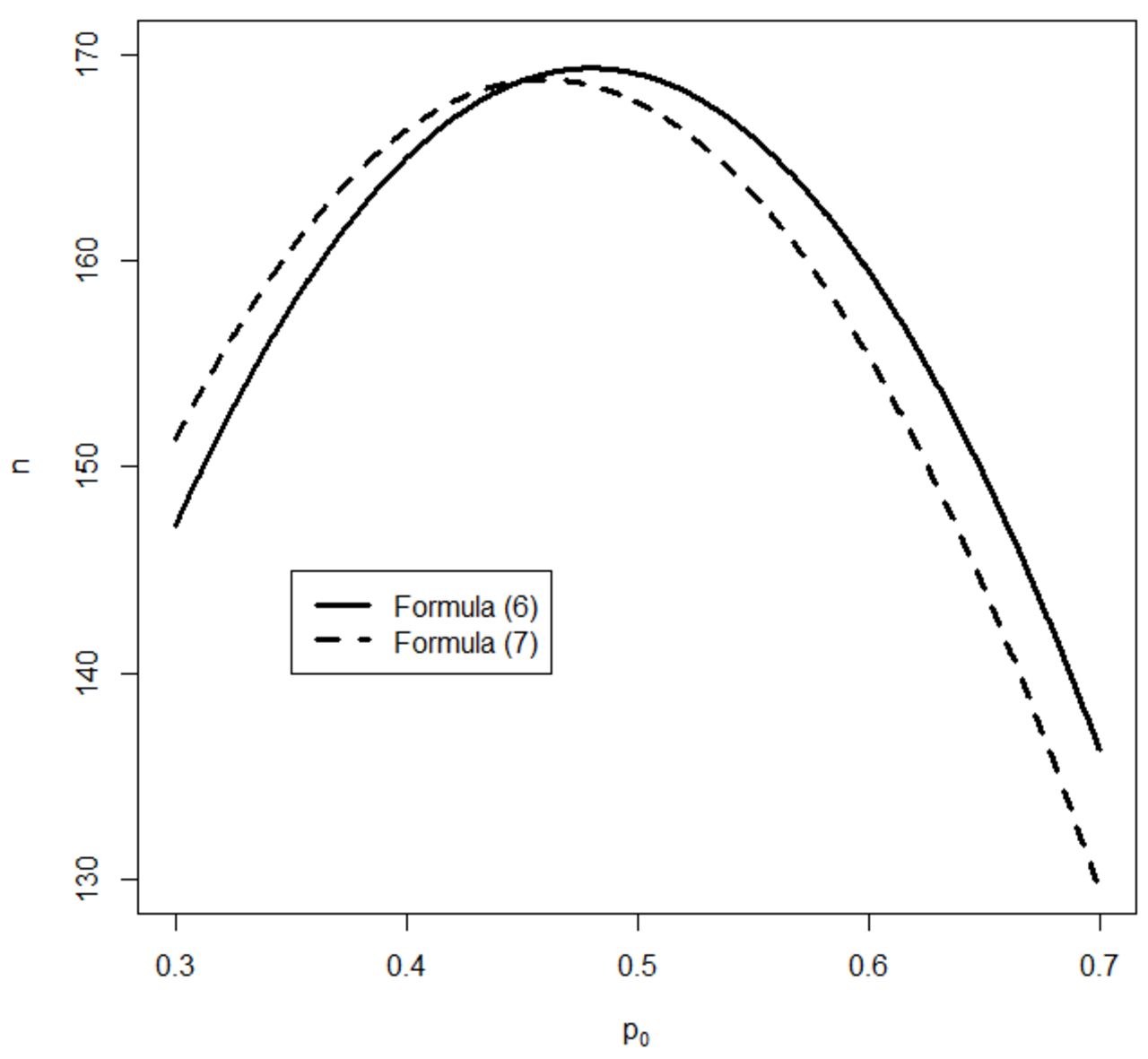
Figure 1 shows the sample size formulas equations 6 and 7 for different  with
with  . Note that in the sample size calculation of Chow and colleagues 3 they did not use the fact that
  in calculating the variance of
  under the null hypothesis.

Sample sizes based formulas (6) and (7).
Sample size based on relative risk
The null and alternative hypotheses are:

where
r
is a known constant. Without loss of generality, assume  .
.
From 6 if we only need new Δ and  to obtain the sample size formula. Given relative risk and
  , the proposed risk difference is:

The new  is:
is:

Substituting (Δ, c 1) into equation 6, we obtain the required sample size based on relative risk.
Sample size based on ORs
The null and alternative hypotheses are

where
θ
is a known constant. Without loss of generality, assume  . The risk difference is

The new  is:
is:

Substituting (Δ, c 1) into equation 6, we obtain the required sample size based on OR.
Conclusion
In this paper, we derive new formulas to calculate sample size based on three popular indices of difference of success rates in two treatment groups. Generally, we cannot uniquely determine the sample size only given one of the risk difference indices. We need the success rates of both groups under the alternative hypothesis. This is usually done through the specification of the success rate of the control group and the difference of two groups. The easiest one is to specify the absolute risk difference Δ between the two groups. If the difference between the two groups is specified by the risk ratio or OR, we can easily transfer them to risk difference Δ and use formula 6 to calculate the sample size.
Figure 1 shows that the sample size calculated based on our formula is generally different than that reported in Chow and colleagues. 3 We compare the accuracies of those two formulas by comparing the powers under different situations. This work is on-going.
Hongyue Wang obtained her BS in Scientific English from the University of Science and Technology of China (USTC) in 1995, and PhD in Statistics from the University of Rochester in 2007. She is a Research Associate Professor in the Department of Biostatistics and Computational Biology at the University of Rochester Medical Center. Her research interests include longitudinal data analysis, missing data, survival data analysis, and design and analysis of clinical trials. She has extensive and successful collaboration with investigators from various areas, including Infectious Disease, Nephrology, Neonatology, Cardiology, Neurodevelopmental and Behavioral Science, Radiation Oncology, Pediatric Surgery, and Dentistry. She has published more than 80 statistical methodology and collaborative research papers in peer-reviewed journals.

Footnotes
Contributors CF and HW derived the theoretical results; BW and JL constructed the examples and graphs; and XMT drafted the manuscript.
Competing interests None declared.
Patient consent Not required.
Provenance and peer review Commissioned; internally peer reviewed.
Data sharing statement No additional data are available.