Article Text

Abstract
For moderate to large sample sizes, all tests yielded pvalues close to the nominal, except when models were misspecified. The signed-rank test generally had the lowest power. Within the current context of count outcomes, the signed-rank test shows subpar power when compared with tests that are contrasted based on full data, such as the GEE. Parametric models for count outcomes such as the GLMM with a Poisson for marginal count outcomes are quite sensitive to departures from assumed parametric models. There is some small bias for all the asymptotic tests, that is,the signed-ranktest, GLMM and GEE, especially for small sample sizes. Resampling methods such as permutation can help alleviate this.
- biostatistics
- statistics as topic
- epidemiologic methods
- investigative techniques
- analytical, diagnostic and therapeutic
This is an Open Access article distributed in accordance with the Creative Commons Attribution Non Commercial (CC BY-NC 4.0) license, which permits others to distribute, remix, adapt, build upon this work non-commercially, and license their derivative works on different terms, provided the original work is properly cited and the use is non-commercial. See: http://creativecommons.org/licenses/by-nc/4.0
Statistics from Altmetric.com
- biostatistics
- statistics as topic
- epidemiologic methods
- investigative techniques
- analytical, diagnostic and therapeutic
Introduction
Although not as popular as continuous and binary variables, count outcomes arise quite often in clinical research. For example, number of hospitalisations, number of suicide attempts, number of heavy drinking days and number of packs of cigarettes smoked per day are all popular count outcomes in mental health research. Studies yielding paired outcomes are also popular. For example, to evaluate new eye-drops, we can treat one eye of a subject with the new eye-drops and the other eye with a placebo drop. To evaluate skin cancer for truck drivers, we can compare skin cancer on the left arm with the right arm, since the left arm is more exposed to sunlight. To evaluate the stress of combat on Veterans’ health, we may use twins in which one is exposed to combat and the other is not, as differences observed with respect to health are likely attributable to combat experience. In a pre-post study, the effect of an intervention is evaluated by comparing a subject’s outcomes before (pre) and after (post) receiving the intervention. In all these studies, each unit of analysis has two outcomes arising from two different conditions. Interest is centred on the difference between the means of the two outcomes.
For continuous outcomes, the paired t-test is the standard statistical method for evaluating differences between the means. However, the paired t-test does not apply to non-continuous variables such as binary and count (frequency) outcomes. For binary outcomes, McNemar’s test is the standard. For count or frequency outcomes, there is not much discussion in the literature. Many use Wilcoxon’s signed-rank test because this method is applicable to paired non-continuous outcomes such as count responses. One major weakness of the signed-rank test is its limited power. As observations are converted to ranks and only ranks are used in the test statistic, the signed-rank test does not use all available information in the original data, leading to lower power when compared with tests that use all data. This is why t-tests are preferred and widely used to compare two independent groups for continuous outcomes.
With recent advances in statistical methodology, there are more options for comparing paired count responses. In this paper, we discuss some alternative procedures that use all information in the original data and thus generally provide more power than the signed-rank test. In the second section, we first provide a brief review of paired outcomes and methods for comparing continuous and binary paired outcomes. We then discuss the classic signed-rank test and modern alternatives for comparing paired count outcomes. In the third section, we compare different methods for comparing paired count outcomes using simulation studies. In the fourth section, we present our concluding remarks.
Methods for paired count outcomes
Paired continuous and binary outcomes
Consider a sample of n subjects indexed by i and let  and
and  denote the paired outcomes from the ith subject. The subject may be an individual or a pair of twins, depending on applications. For example, in a pre-post study, the paired outcomes correspond to the pretreatment and post-treatment assessment and the subject is an individual. In studies involving twins, the paired outcomes come from each pair of twins. Because the two outcomes are correlated, statistical methods for comparing independent samples such as the t-test cannot be applied.
For a continuous outcome, the paired t-test is generally applied to evaluating differences in the means of the paired outcomes. If we assume that  and
and  follow a bivariate normal distribution, then the difference between the two outcomes,
  , is also normally distributed. Under the null of no difference between the means of the two outcomes,
  has a normal distribution with mean
0
and variance
has a normal distribution with mean
0
and variance  . Thus, we can apply the t-test to the differences
  to test the null:
 (1)
(1)
where  denotes the t distribution with k df, and
  and
and  denote the sample mean and SD. We can also use this sampling distribution to construct CIs.
In practice, the bivariate normal distribution assumption for the paired outcomes  and
and  is quite strong and may not be met in real study data. If the assumption fails, the differences
  generally do not follow the normal distribution and thus the
  statistic in Equation (1) may not follow the t distribution. For large samples such as
  ,
,  follows approximately a standard normal distribution. Thus, one may replace
  with the ‘asymptotic’ standard normal,
  , to test the null as well as construct CIs, even if the outcomes
  and
and  are not bivariate normal.
In what follows, we assume large samples, since all the tests to be discussed next are asymptotic tests, that is, they approximately follow a mathematical distribution such as the normal distribution only for large samples. For small to moderate samples, all these tests have unknown distributions and asymptotic mathematical distributions such as the standard normal for large samples for the paired t-test may not work well. We discuss alternatives for small to moderate samples in the discussion section.
If the paired outcomes are binary, the above hypothesis becomes the comparison of the proportions of  and
and  . McNemar’s test is the standard for comparing the paired outcomes. Let
  and
and  denote the proportions associated with
  and
and  , that is,

Then the hypothesis to be tested is given by:
 (2)
(2)
McNemar’s test is premised on the idea of comparing concordant and discordant pairs in the sample.
Shown in table 1 is a  cross-tabulation for the two levels of the binary outcomes. Let
  ,
,  ,
,  and
and  denote the cell probabilities (or proportions) for the four cells in the table, that is,
A 2×2 contingency table displaying joint distributions of paired binary outcomes, with a, b, c and d denoting cell count

Then,  can be expressed in terms of the cell probabilities as follows:

Similarly,  can be expressed as:

Thus,  implies
  and vice versa. The hypothesis of interest in Equation (2) involving
  and
and  can be expressed in terms of
  and
and  :
:

McNemar’s test evaluates the difference between the concordant and discordant pairs, b and c, that is,
A large difference leads to rejection of the null. By normalising this difference, the statistic  above follows approximately the standard normal for large sample size.
Paired count outcomes
For count outcomes, McNemar’s test clearly does not apply. The paired t-test is also inappropriate for such outcomes. First, the difference  does not follow a normal distribution. Second, even if both
  and
and  follow a Poisson distribution, the difference
  is not a Poisson variable;
  in general is not even guaranteed to have non-negative values.
One approach that has been used to compare paired count outcomes is the Wilcoxon signed-rank test. Within our context, let  denote the rank of
  based on its absolute value
  . The ranks are integers that indicate the position of
  after rearranging them in ascending order.1 The signed-rank test has the following statistic:
where  denotes an indicator with the value 1 (0) if the logic
  >0 is true (otherwise). Thus,
  only adds up the ranks for the positive
  ’s.
’s.
The statistic  ranges from 0 to
  . Under
  , about one-half of the
  's are positive. Thus, any pair (
 ,
,  ) has 50% chance that
  . In terms of ranks, this means that the sum of
  for positive
  is about half of the range
  . Thus, we can specify the null as:
where  . Under the null
  ,
,  has mean
  , half of the range
  . The normalised
  :
:
 (3)
(3)
has approximately a normal distribution with mean  and SE
  for large samples, which is readily applied to calculate p values and/or confidence bands.
Since paired outcomes are a special case of general longitudinal outcomes, longitudinal methods can be applied to test the null. For example, both the generalised linear mixed-effects model (GLMM) and generalised estimating equations (GEE), two most popular longitudinal models, can be specialised to the current setting. When applying GLMM, we specify the following model:
 (4)
(4)
where z denotes a random effect to account for correlation between the paired outcomes,  denotes a Poisson distribution with mean
μ
,
denotes a Poisson distribution with mean
μ
,  denotes the exponential and
  denotes the log function. The null of same mean between
  and
and  can be expressed as:

Note that since the random effect z may be positive or negative and the random of the normal distribution is unbounded, the log transformation of the Poisson mean in Equation (4) is necessary to ensure that  and
and  stay positive.
For applying GEE, we only need to specify the mean of each paired outcome. This is because unlike GLMM, GEE is a ‘semi-parametric’ model and imposes no mathematical distribution on the outcomes. Thus, under GEE, both the Poisson distribution for each outcome and the random effect z for linking the paired outcomes are removed. The corresponding GEE is given by:
 (5)
(5)
Since there is no random effect in Equation (5), the log transformation is also not necessary and thus the GEE can be specified simply as:
 (6)
(6)
Compared with the GLMM in Equation (4), the GEE above imposes no mathematical distribution either jointly or marginally, allowing for valid inference for a broad class of data distributions. The GLMM in Equation (4) may yield biased inference if: (1) at least one of the outcomes does not follow the Poisson; (2) the random effect z follows a non-normal distribution; and (3)  and
and  are not correlated according to the specified random-effect structure. In contrast, the GEE in Equation (5) forgoes all such constraints and yields valid inference regardless of the marginal distribution and correlation structure of the outcomes
  and
and  .
.
Simulation study
In this section, we evaluate and compare the performances of the different methods discussed above by simulation. All simulations are performed with a Monte Carlo (MC) sample of  under a significance level of
  . Performance of a test is characterised by: (1) bias and (2) power. We consider both aspects when comparing the different methods.
Bias
If a test performs correctly, it should yield type I error rates at the specified nominal level  . Several factors can affect the performance of the test. First, if data do not follow the assumed mathematical distributions, the test in general is biased. For example, if the paired t-test is applied to paired outcomes that are not bivariate normal, it will generally be biased. Second, with the exception of the paired t-test, all tests discussed above rely on large samples to provide valid results. When applied to small or moderate samples, such tests may have bias. For example, the normal distribution may not provide a good approximation to the sampling distribution of the statistic
  of the Wilcoxon signed-rank test
  when applied to a sample size of, say,
  . Thus, to compare the performance of each different method, we consider sample sizes ranging from n= 10 to 200.
To evaluate the effects of model assumptions on test performance, we simulate correlated count responses  and
and  using a copula approach,2 where each outcome marginally follows a negative binomial (NB) distribution:
 (7)
(7)
The above model deviates from the GLMM in Equation (4) in two ways. First,  (
( ) follows an NB, rather a Poisson. Second, correlation between
  and
and  does not follow the normal distribution based on random effect. Unlike Poisson, NB has an extra parameter
τ
controlling for dispersion (variability). Thus, although Poisson and NB have the same mean, NB has a different (larger) variance than Poisson.1 Since
does not follow the normal distribution based on random effect. Unlike Poisson, NB has an extra parameter
τ
controlling for dispersion (variability). Thus, although Poisson and NB have the same mean, NB has a different (larger) variance than Poisson.1 Since  converges to
  as
τ
increases, selecting a relatively small
τ
allows us to examine the impact of the Poisson assumption on inference when the GLMM in Equation (4) is applied to count outcomes that are not compliant with the Poisson model.
as
τ
increases, selecting a relatively small
τ
allows us to examine the impact of the Poisson assumption on inference when the GLMM in Equation (4) is applied to count outcomes that are not compliant with the Poisson model.
For the simulation study, we set  and 5, and correlation between
  and
and  to 0.5. To evaluate bias using MC simulation, we simulate paired outcomes
  and
and  from the model in Equation (7), apply each of the tests discussed in the third section and compute p values for testing the null hypothesis. This process is repeated
  times. A test has little or no bias if the proportion of nulls rejected over the
  times is close to the nominal value
  .
.
Shown in table 2 are averaged p values for the different tests from their applications to the  simulated paired outcomes, where GLMM (Poisson) denotes the GLMM for Poisson in Equation (4), GLMM (NB) denotes the GLMM for NB distribution (by replacing the Poisson in the GLMM in Equation (4) with NB), GEE denotes the GEE without log transformation in Equation (6) and GEE (log-link) denotes the GEE with log transformation in Equation (5). For moderate to large sample sizes, n=100, 200, all tests yielded p values close to the nominal
  , except for GLMM (Poisson), which had highly inflated type I errors for
  . As indicated earlier, with a small dispersion parameter such as
  , NB has much more variability than its Poisson counterpart, leading to poor fit when fitting simulated data with the GLMM assuming the Poisson. Thus, the high bias in the type I error reflects model mis specification.
Averaged p values from testing the null of no difference between paired outcomes by different methods over M=2000 MC replicates
Although the paired t-test is not a valid test, it performed well for all sample sizes considered, although showing small downward bias, especially for small sample sizes. For extremely small sample sizes such as n=10, all three asymptotically valid methods, signed-rank test, GLMM (NB) and GEE, showed small upward bias, especially when  . As the sample size increased, the bias diminished, as expected.
Power
If a group of tests all provide good type I error rates, we can further compare them for power. It is common that two unbiased tests may provide different power, because they may use a different amount of information from study data or use the same information differently. For example, within the current study, the signed-rank test may provide less power than the GEE, because the former only uses the ranks of the original count outcomes, completely ignoring magnitudes of  ’s. Thus, it is of interest to compare power across the different tests.
We again use the MC approach to compare power across the different methods. However, unlike the evaluation of bias, we must also be specific about the difference in the means of paired outcomes so that we can simulate the outcomes under the alternative hypothesis. For this study, we specify the null and alternative as follows:
 (8)
(8)
We simulate correlated outcomes  again using the copula from the GLMM in Equation (7), but with
  and
and  as specfied under
  in Equation (8).
For each simulated outcome  , we apply the different methods and test the null hypothesis under
  . This process is repeated
  times and the power for each method is estimated by the per cent of times the null is rejected.
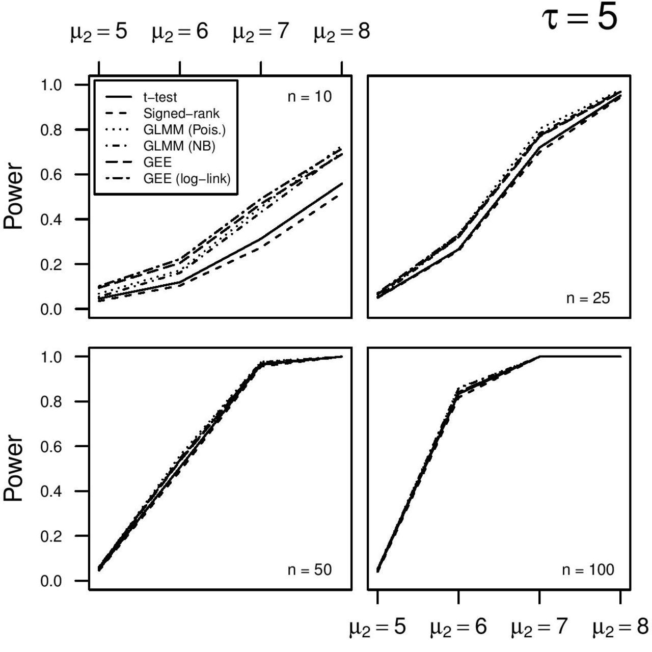
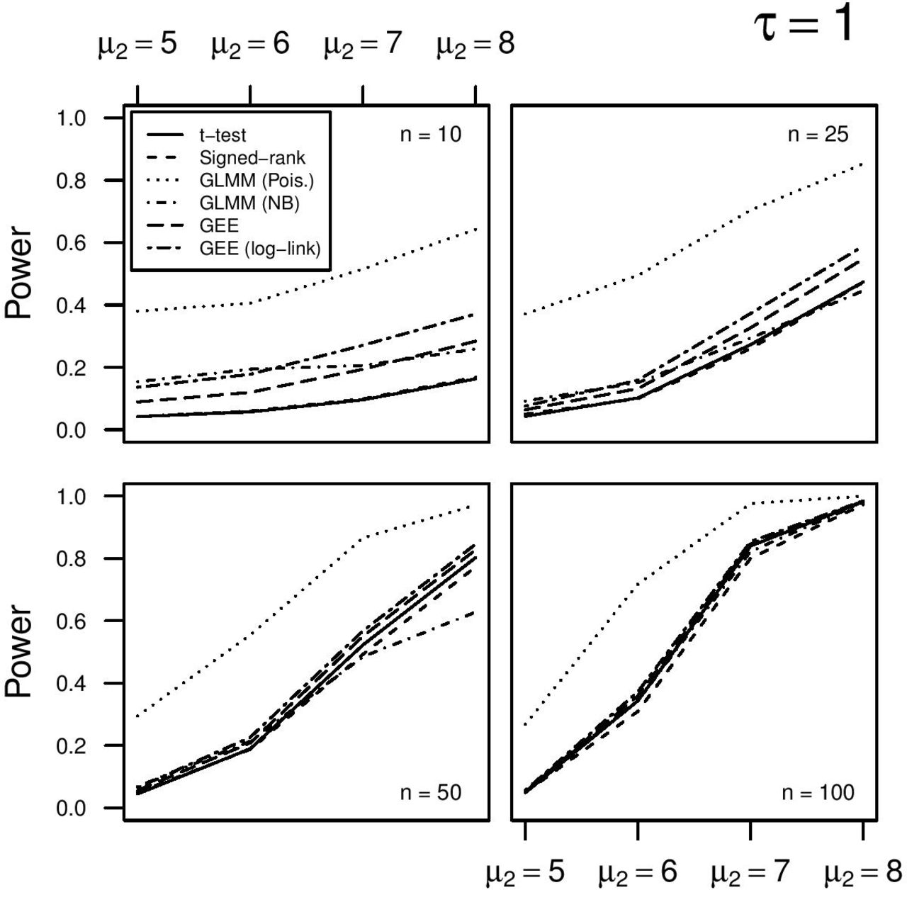
Shown in table 3 are power estimates from testing the null hypothesis in Equation (8) by the different methods from their applications to the  paired count outcomes simulated under the alternative hypothesis in Equation (8). As type I error rates for GLMM (Poisson) were highly biased, power estimates from this method are not meaningful. Among the remaining four tests, the signed-rank test has the lowest power. The paired t-tests, GLMM (NB) and both GEE methods yield comparable power estimates, though both GEE methods and GLMM (NB) appear to perform best with a sample size of at least 25. When
  and the sample size is high (more than, say, 50 subjects) all tests have comparable power and correct nominal significance level. Figures 1 and 2 show the power estimates under additional alternative hypotheses. The GLMM (NB) method appears to be less efficient for larger differences in means with sample sizes around 50 when
  .
.
Power estimates from testing the null of no difference between paired outcomes by different methods over M=2000 MC replicates

Power for each method under different alternative hypotheses. Data are generated with larger dispersion (ie,  ). GEE, generalised estimating equation; GLMM, generalised linear mixed-effects model; NB, negative binomial.
Power for each method under different alternative hypotheses. Data are generated with smaller dispersion (ie,  ), more similar to a Poisson distribution. GEE, generalised estimating equation; GLMM, generalised linear mixed-effects model; NB, negative binomial.
Discussion
In this report, we discussed several methods for testing differences in paired count outcomes. Unlike paired continuous and binary outcomes, analysis of paired count outcomes has received less attention in the literature. Although the signed-rank test is often used, it is not an optimal test. This is because it uses ranks, rather than original count outcomes (differences between paired count outcomes), resulting in loss of information and leading to reduced power. Thus, unless study data depart severely from the normal distribution, the signed-rank test is not used for comparing paired continuous outcomes, as the paired t-test is a more powerful test. Within the current context of count outcomes, the signed-rank test again shows subpar power when compared with tests that are contrasted based on full data, such as the GEE.
The simulation study in this report also shows that parametric models for count outcomes such as the GLMM with a Poisson for marginal count outcomes are quite sensitive to departures from assumed parametric models. As expected, semiparametric models like the GEE provide better performance. Also, the paired t-test seems to perform quite well. This is not really surprising, since within the current context the GEE and paired t-test are essentially the same, except that the former relies on the asymptotic normal distribution for inference, while the latter uses the t distribution for inference. As the sample size grows, the t becomes closer to the standard normal distribution. Thus, p values and power estimates are only slightly different between the two for small to moderate samples.
The simulation results also show some small bias for all the asymptotic tests, that is, the signed-rank test, GLMM and GEE, especially for small sample sizes. In most clinical studies, sample sizes are relatively large and this limitation has no significant impact. For studies with small samples, such as those in bench sciences, bias in type I error rates may be high and require attention. One popular statistical approach is to use resampling methods such as permutation.3 Within the current context of paired count responses, the permutation technique is readily implemented. For example, we first decide whether to switch the order of the paired outcomes  in a random fashion and then apply any of the tests considered above, such as the GEE, and compute the statistic based on the ‘permuted’ sample. We repeat this process M times (such as M=1000) and obtain a sampling distribution of the test statistic. If the statistic based on the original data falls either below the 2.5th or above the 97.5th percentile, we reject the null. Under permutation, model assumptions such as the Poisson in the GLMM have no impact on inference and all the tests provide valid inference.
Supplemental material
James Proudfoot obtained a master’s degree in statistics from the University of British Columbia. He is currently in the Biostatistical and Epidemiology Research Division at UC San Diego, CA. His work involves manuscripts preliminary assessment, biostatistical analysis counseling, and research on the application of statistical methods in psychiatric studies.

Footnotes
Contributors JAP directed all simulation studies, ran some of the simulation examples and helped edit and finalise the manuscript. TL helped run some of the simulation examples and drafted some parts of the manuscript. BW helped check some of the simulation study results and draft part of the simulation results. XMT helped draft and finalise the manuscript.
Funding The report was partially supported by the National Institutes of Health, Grant UL1TR001442 of CTSA funding.
Disclaimer The content is solely the responsibility of the authors and does not necessarily represent the official views of the NIH.
Competing interests None declared.
Patient consent Not required.
Provenance and peer review Not commissioned; externally peer reviewed.
Data statement No additional data are available.